43 data labels excel pie chart

Display data point labels outside a pie chart in a paginated report ... Create a pie chart and display the data labels. Open the Properties pane. On the design surface, click on the pie itself to display the Category properties in the Properties pane. Expand the CustomAttributes node. A list of attributes for the pie chart is displayed. Set the PieLabelStyle property to Outside. Set the PieLineColor property to Black. Change the format of data labels in a chart To format data labels, select your chart, and then in the Chart Design tab, click Add Chart Element > Data Labels > More Data Label Options. Click Label Options and under Label Contains, pick the options you want. To make data labels easier to read, you can move them inside the data points or even outside of the chart.

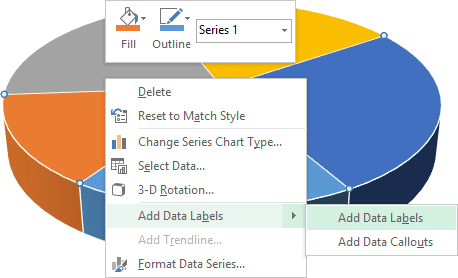
Pie Chart in Excel | How to Create Pie Chart - EDUCBA Example #2 - 3D Pie Chart in Excel Step 1: . Select the data to go to Insert, click on PIE, and select 3-D pie chart. Step 2: . Now, it instantly creates the 3-D pie chart for you. Step 3: . Right-click on the pie and select Add Data Labels. This will add all the values we are showing on the ...

Data labels excel pie chart

Adding data labels to a Pie Chart in VBA - Automate Excel Adding data labels to a Pie Chart in VBA - Automate Excel. Office: Display Data Labels in a Pie Chart - Tech-Recipes 2. If you have not inserted a chart yet, go to the Insert tab on the ribbon, and click the Chart option. 3. In the Chart window, choose the Pie chart option from the list on the left. Next, choose the type of pie chart you want on the right side. 4. Once the chart is inserted into the document, you will notice that there are no data labels. How to Make a Pie Chart in Excel (Only Guide You Need) How to Insert Data into a Pie Chart in Excel. The first condition of making a pie chart in Excel is to make a table of data. In this example, we will see the process of inserting data from a table to make a pie chart. Here we will be analyzing the attendance list of 5 months of some students in a course. The table s given below.

Data labels excel pie chart. How do you label data points in Excel? - profitclaims.com 1. Right click the data series in the chart, and select Add Data Labels > Add Data Labels from the context menu to add data labels. 2. Click any data label to select all data labels, and then click the specified data label to select it only in the chart. 3. Excel Date Pie Chart - TheRescipes.info How to Create and Format a Pie Chart in Excel - Lifewire tip . Jan 23, 2021To create a pie chart, highlight the data in cells A3 to B6 and follow these directions: On the ribbon, go to the Insert tab. Select Insert Pie Chart to display the available pie chart types. Hover over a chart type to read a description of the chart and to preview the pie chart. › comparison-chart-in-excelComparison Chart in Excel | Adding Multiple Series Under Same ... This window helps you modify the chart as it allows you to add the series (Y-Values) as well as Category labels (X-Axis) to configure the chart as per your need. Under Legend Entries ( S eries) inside the Select Data Source window, you need to select the sales values for the year 2018 and year 2019. excelunlocked.com › pie-of-pie-chart-in-excelPie of Pie Chart in Excel - Inserting, Customizing - Excel ... Jan 03, 2022 · In the above example, there were a total of 6 data points. The Parent Pie chart represents three of them i.e Facebook, Youtube, and Instagram while the fourth data point named “Other” splits into a subset Pie chart that represents the rest of the three data points i.e Zee, Linkedin, and Hotstar.

support.microsoft.com › en-us › officeAdd or remove data labels in a chart - support.microsoft.com Data labels make a chart easier to understand because they show details about a data series or its individual data points. For example, in the pie chart below, without the data labels it would be difficult to tell that coffee was 38% of total sales. Depending on what you want to highlight on a chart, you can add labels to one series, all the ... why are some data labels not showing in pie chart ... - Power BI Hi @Anonymous. Enlarge the chart, change the format setting as below. Details label->Label position: perfer outside, turn on "overflow text". For donut charts, you could refer to the following thread: How to show all detailed data labels of donut chart. Best Regards. Creating Pie Chart and Adding/Formatting Data Labels (Excel) Creating Pie Chart and Adding/Formatting Data Labels (Excel) - YouTube. How to Make a Pie Chart in Excel & Add Rich Data Labels to The Chart! Creating and formatting the Pie Chart 1) Select the data. 2) Go to Insert> Charts> click on the drop-down arrow next to Pie Chart and under 2-D Pie, select the Pie Chart, shown below. 3) Chang the chart title to Breakdown of Errors Made During the Match, by clicking on it and typing the new title.

› examples › pie-chartHow to Create Pie Charts in Excel (In Easy Steps) 6. Create the pie chart (repeat steps 2-3). 7. Click the legend at the bottom and press Delete. 8. Select the pie chart. 9. Click the + button on the right side of the chart and click the check box next to Data Labels. 10. Click the paintbrush icon on the right side of the chart and change the color scheme of the pie chart. Result: 11. Adding data labels to a pie chart - Excel General - OzGrid Re: Adding data labels to a pie chart. Thanks again, norie. Really appreciate the help. I tried recording a macro while doing it manually (before my first post). But it didn't record anything about labels, much less making them bold. How to add data labels from different column in an Excel chart? Right click the data series in the chart, and select Add Data Labels > Add Data Labels from the context menu to add data labels. 2. Click any data label to select all data labels, and then click the specified data label to select it only in the chart. 3. Add data labels and callouts to charts in Excel 365 | EasyTweaks.com Step #1: After generating the chart in Excel, right-click anywhere within the chart and select Add labels . Note that you can also select the very handy option of Adding data Callouts. Step #2: When you select the "Add Labels" option, all the different portions of the chart will automatically take on the corresponding values in the table ...

Bar Chart in Excel - Easy Excel Tutorial

Inserting Data Label in the Color Legend of a pie chart Re: Inserting Data Label in the Color Legend of a pie chart @SabrinaFr There is no built-in way to do that, but you can use a trick: see Add Percent Values in Pie Chart Legend (Excel 2010)

Excel 3-D Pie Charts - Microsoft Excel 2013

Pie Chart in Excel - Inserting, Formatting, Filters, Data Labels To add Data Labels, Click on the + icon on the top right corner of the chart and mark the data label checkbox. You can also unmark the legends as we will add legend keys in the data labels. We can also format these data labels to show both percentage contribution and legend:- Right click on the Data Labels on the chart.

How to Show Percentages in Stacked Bar and Column Charts in Excel

data-flair.training › blogs › types-of-charts-in-excelTypes of Charts in Excel - DataFlair 1. Pie Chart in Excel. Pie Chart is one that resembles a Pie. These are mainly used when one wants to represent the data in percentages. Here each data point i.e, the pie shows the respective percentages. Pie charts are best when we have one data series. Types of Pie Chart. The pie chart has the following sub types and they are 2-D pie chart ...

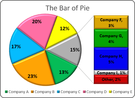
Creating Pie of Pie and Bar of Pie charts - Microsoft Excel 2016

Resize Pie Chart Data Labels - Excel Charting & Graphing - Board ... 2. Type = in the formula bar and click on the. cell that you want to link to the label. Once linked you can explicitly control line. breaks using the CHAR worksheet function (e.g., ="long"&CHAR (10)&"label") or by using the. Alt+Enter key combination while entering the. label (i.e., type "long"; press Alt+Enter;

How to Show Percentages in Stacked Bar and Column Charts in Excel

How to Create a Pie Chart in Microsoft Excel To create a pie chart, you must first enter your data into the Excel spreadsheet. The data should be entered in rows and columns, with one column for the category name and one for the corresponding percentage or value. Once you have your data set up, select the range of cells that contains it and then click on the Insert tab.

410 How to display percentage labels in pie chart in Excel 2016 - YouTube

Microsoft Excel Tutorials: Add Data Labels to a Pie Chart To change this, right click your chart again. From the menu, select Format Data Labels: When you click Format Data Labels , you should get a dialogue box. This one: If there's a tick in Percentage, untick this and select Value: Your chart will then have the correct numbers: Overall, the chart looks OK. But we can add some formatting to it. in the next part, you'll see how to format each individual segement of the Pie Chart.

SQL & BI Learning: Pie Chart with data labels outside in ssrs

Multiple data labels (in separate locations on chart) You can use the Up/Down arrows to move through chart elements in order to select the second pie. Or use the drop down on the charting toolbar to select the 2nd series Attached Files 819208a.xlsx‎ (77.9 KB, 399 views) Download Register To Reply 08-16-2013, 05:58 AM #6 petesurfer Registered User Join Date 04-16-2013 Location London, England

Python matplotlib Pie Chart

How to Create and Format a Pie Chart in Excel - Lifewire Select the plot area of the pie chart. Select a slice of the pie chart to surround the slice with small blue highlight dots. Drag the slice away from the pie chart to explode it. To reposition a data label, select the data label to select all data labels. Select the data label you want to move and drag it to the desired location.

Share :